A differentiable Turing machine the internal program of which can thus be learned. The program can be represented using Artificial neural networks. A Neural Turing Machine (NTM) architecture contains two basic components: a neural network controller and a memory bank
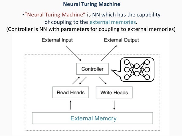
Neural Turing Machines. It emulates working Memory in the Brain
Key aspects
- Recurrent neural networks for the controller, and read write heads. Often Long short-term memory
- Memory
- Addressing system that implements Attention, and is differentiable.
It can learn basic Algorithms, and thus it's a form of Program induction. It also addresses the Binding problem and the problem of computing with variable-length structures, both of which had been studied before. These are important steps to address towards creating General artificial intelligence.
Crucially, every component of the architecture is differentiable, making it straightfor- ward to train with gradient descent. We achieved this by defining ‘blurry’ read and write operations that interact to a greater or lesser degree with all the elements in memory (rather than addressing a single element, as in a normal Turing machine or digital computer)
Symposium: Deep Learning - Alex Graves
See Integrating symbols into deep learning, Neural networks with memory, Augmented RNN
Also see Neural programmer-interpreter
Reading
The read weights vector , is outputted by the read head. These are multiplied with the memory locations to give the read vectors.
Writting
A set of vectors with elements in the range is outputted by the write head.
- An attention write weight vector,
- An erase vector
- An add vector
Algorithm:
- Update each memory location from the previous time by , where is a row vector of all 1s, and the multiplication against the memory location acts pointwise.
- Adding the add vector:
Addressing mechanism
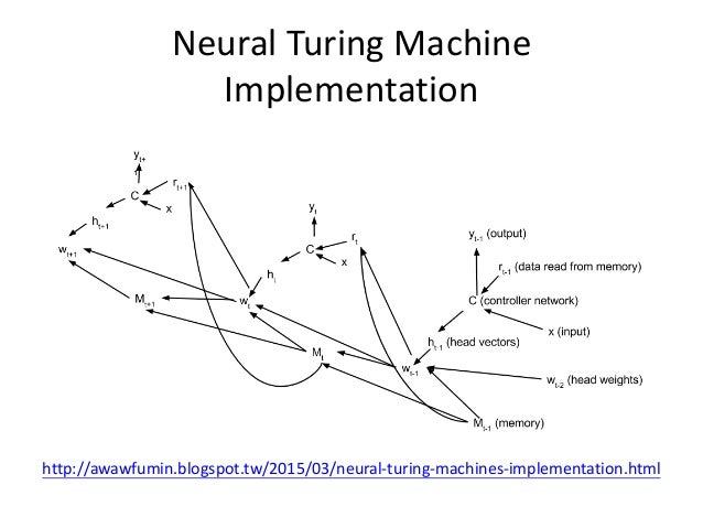
See here for interactive version. This diagram is missing a few variables used in the NTM defined on the paper. See below for fuller diagram.

Two combined addressing mechanisms:
- "content-based addressing,” focuses attention on locations based on the similarity between their current values and values emitted by the controller. See Focusing by content on paper
- "location-based addressing". In certain tasks the content of a variable is arbitrary, but the variable still needs a recognisable name or address. Loops are an example of where we need this. See Focusing by location on paper
Content-based addressing is strictly more general than location-based addressing as the content of a memory location could include location information inside it. In our ex- periments however, providing location-based addressing as a primitive operation proved essential for some forms of generalisation, so we employ both mechanisms concurrently.
Controller
Advantages and disadvantages of feedforward vs recurrent (LSTM) controller network. With a single read head, it can perform only a unary transform on a single memory vector at each time-step, with two read heads it can perform binary vector transforms, and so on. Recurrent controllers can internally store read vectors from previous time-steps, so do not suffer from this limitatio
Experiments
The hallmark of such solutions is that they generalise well beyond the range of the training data
copy,
learns to copy onto memory, go back to beginning (using associative memory), and iterate over memory printing result, using the relative, location-based memory addressing mechanism
repeat copy,
learns to store the number of times it needs to repeat.
Whereas LSTM fails both tests, NTM succeeds with longer sequences and is able to perform more than ten repetitions; however it is unable to keep count of of how many repeats it has completed, and does not predict the end marker correctly. This is probably a consequence of representing the number of repetitions numerically, which does not easily generalise beyond a fixed range
associative recall
The next order of complexity in organising data arises from “indirection”—that is, when one data item points to another. We test the NTM’s capability for learning an instance of this more interesting class by constructing a list of items so that querying with one of the items demands that the network return the subsequent item
Figure 10 shows that NTM learns this task significantly faster than LSTM, terminating at near zero cost within approximately 30, 000 episodes, whereas LSTM does not reach zero cost after a million episodes. makes sense as the architecture of the NTM seems much more tuned for this task.
Dynamic n-grams
The goal of the dynamic N-Grams task was to test whether NTM could rapidly adapt to new predictive distributions. In particular they wanted to test if it could use its memory as a re-writable table that it could use to keep count of transition statistics, thereby emulating a conventional N-Gram model.
The network observes the sequence one bit at a time and is then asked to predict the next bit. NTM achieves a small, but significant performance advantage over LSTM, but never quite reaches the optimum cost. Close analysis of NTM’s memory usage (Figure 15) suggests that the controller uses the memory to count how many ones and zeros it has observed in different contexts, allowing it to implement an algorithm similar to the optimal estimator.
Priority sort
This task tests whether the NTM can sort data—an important elementary algorithm. A sequence of random binary vectors is input to the network along with a scalar priority rating for each vector. The priority is drawn uniformly from the range [-1, 1]. The target sequence contains the binary vectors sorted according to their priorities
memory use led us to hypothesise that it uses the priorities to determine the relative location of each write. T
Note that eight parallel read and write heads were needed for best performance with a feedforward controller on this task; this may reflect the difficulty of sorting vectors using only unary vector operations (see Section 3.4).
What Sorting algorithm is it using? From pictures I think it sorts while writing, and then reads in sequence. But how does it sort it anyway?