See MMathPhys oral presentation.

Theoretical framework

Following The Arrival of the Frequent: How Bias in Genotype-Phenotype Maps Can Steer Populations to Local Optima (remember notes here are complementary to paper, and don't cover all of its content, only those parts where I thought were gaps for me to understand it), we can study the effect of the structure of the genotype-phenotype (GP) map, in the model of Evolution known as the Wright-Fisher model (see Population genetics). We use the Haploid Wright-Fisher model with selection, where for each individual in the generation at time $t+1$, we choose a single parent from the individuals at the previous generation $t$, according to the rule described there. We then include the effect of mutations, by assigning to the new individual a genotype of length $L$ as follows:

• Copy the genotype of parent.
• For each of the letters in the genotype, replace it with probability $\mu$, the point mutation rate. When you replace, you replace it by a different letter, chosen uniformly at random from the different letters.

Note: the genotype is defined as a sequence of $L$ letters taken from an alphabet of $K$ letters.

See Mean field approximation to average number of phenotypes discovered in Wright-Fisher model , some equations are found there. The main result is that the expected number of individuals with genotype $p$ that arises at generation $t$ can be approximated as

under certain assumptions, explained in that tiddler.

Polymorphic limit

If $NL\mu \gg 1$, the population naturally spreads over different genotypes, a regime called the polymorphic limit. See Polymorphic limit (Wright-Fisher model) tiddler for details. Main points:

To model neutral exploration, we let $1+s_p = \delta_{pq}$, where $\delta_{pq}$ is a Kronecker delta

The time when {{the probability of having discovered a p-type individual (produced a p-type offspring)} is $\alpha$} is found by:

Monomorphic limit

Neutral spaces can be astronomically large, much bigger than even the largest viral or bacterial populations (see this paper). In that case, the local neighborhood of the population may not be fully representative of the neighborhood of the entire space.

This scenario can most easily understood in the monomorphic limit: when mutants are rare, $NL \mu \ll 1$

Now, the (average) rate of neutral mutations (per individual) is $\nu = L \mu \rho$, as $\rho$ is the probability that a mutation is neutral.

See more in the Monomorphic limit (Wright-Fisher model) tiddler, and at the paper.

We can see that in the large genome limit, the phenotype $p$ is found quicker as the population $N$ increases. However, when the population becomes so large that all the 1-mutation neighbourhood is thoroughly explored (while still staying in the monomorphic limit), the discovery time saturates because increasing the population doesn't increase the number of explored phenotypes (during a fixation period).

These results suggest that for intermediate $NL\mu$ there should be a smooth transition between these two regimes. To quantify the crossover we introduce a factor $\gamma$.

[See Figure 1.]

Simulations in model GP maps

The genotype is defined by:

• Alphabet length: $K$
• Genotype length: $L$

The number of available genotypes is thus $K^L$.

Random GP map:

Apart from specifying $K$ and $L$, we need to specify the set $\{F_q\}$ which is the fraction of genotypes mapping to phenotype $p$. The map is otherwise random.

In this setting, $\phi_{pq} = F_p$ is a good approximation if $N_q, N_p \gg 1$, where $N_i$ is the number of genotypes mapping to phenotype $i$. These also require $N_P \ll N_G$ (i.e. {the number of phenotypes } is much less than {the number of genotypes}, i.e the map is very many-to-one).

There is also a percolation threshold at a critical frequency ($F_p$) $\lambda(K) = 1 - K^{-1/(K-1)}$, so that only phenotypes with $F_p > \lambda(K)$ have "completely" connected neutral spaces (in the network where edges correspond to a single-point mutations, or genotypes separated by a Hamming distance of $1$). See the theory of percolation in Network science's Newman's book, Oxford notes, and problem sheets. See also Random Induced Subgraphs of Generalized n-Cubes.

Standing variation. Adaptation from standing genetic variation.

RNA secondary structure mapping

RNA genotypes of length $L$ made up of nucleotides G,C,U and A.

The phenotypes are the minimum free-energy secondary structures for the sequences, which can beefficiently calculated (see Fast Folding and Comparison of RNA Secondary Structures). The number of genotypes grows as $4^L$,while the number of phenotypes is thought to grow roughly as $N_P \sim 1.8^L$ (see Robustness and Evolvability in Living Systems - Andreas Wagner). Also:

From sequences to shapes and back: a case study in RNA secondary structures. - pdf.

Epistasis can lead to fragmented neutral spaces and contingency in evolution

The Ascent of the Abundant: How Mutational Networks Constrain Evolution

Discovery times are slower than in the random GP map. This reflects the internal structure of the RNA: similar genotypes typically have similar mutational neighbourhoods (see Exploring phenotype space through neutral evolution.), and so the population needs to neutrally explore longer in order to find novelty.

Phenotypic bias leads to a simple, systematic ordering in the discovery of novel phenotypes.

The arrival of the frequent

Comment: The fact that this discussion requires speaking about a change in the environment is what makes "the arrival of the frequent" a non-equilibrium effect, I think. Compare this with the survival of the flattest which is an equilibrium effect.

We need to have $s2, s_1\gtrsim 1/(2N)$ because the probability of fixation is (see here (page 201) or here, or here (page 326)):

$P = \frac{1-e^{-qs}}{1-e^{-2Ns}}$

So for $2Ns \gtrsim 1$, $\frac{q(2Ns)}{2N(1-e^{-(2Ns)})} > \frac{q}{2N}$. We need to have $s2, s_1\gtrsim 1/(2N)$ so that the probability of fixation of the two alternative phenotypes is considerably larger than that of the initial phenotype $q$, for which $s=0$. In here (page 321) an expression for the case of $N$ very large is derived without using diffusion approximation.

A more frequent phenotype ($p1$, with $\phi_p1q$ much larger than competitor $p2$) is favoured via two related effects:

• It is discovered much earlier, and so it has a chance to fix before $p2$.
• Because the discovery time-scale is much smaller, if {we are in the large population monomorphic limit, so that the single-mutation neighbourhood is explored many times before population fixes to a new genotype}, then $p1$ is also visited more often. Therefore its fixation probability is larger. Say that $p1$ is visited $n$ times, then the probability that it fixes is $1-(1-p)^n \approx np$, where $p$ is the probability that it fixes when it's visited once ($1/N$ without selection bias), and it is much smaller than $1$ for the approximation ($N$ large). >Isn't this the same as the result that "The rate of fixations is equal to the rate of (neutral) mutations of an individual." derived in Monomorphic limit (Wright-Fisher model)? Yes.This is observed in their microscopic models (On the significance of neutral spaces in adaptive evolution). This effect is ignored in origin-fixation models (see Bias in the introduction of variation as an orienting factor in evolution) Hm, how exactly is it ignored? haven't read the paper yet... Well, from what Ard said, the way they ignore is that they ignore the short-time correlations in the monomorphic limit, discussed in the paper.

Another effect that often positively correlates with the frequency of a phenotype is Mutational robustness (see Robustness and evolvability: a paradox resolved and Epistasis can lead to fragmented neutral spaces and contingency in evolution). Mutational robustness has been shown to offer selective advantage at high mutation rates, because phenotypes which are not robust will often mutate to deleterious mutants and probably go extinct, while phenotypes which are robust will survive. This effect is called the "survival of the flattest", as robust phenotypes correspond to "flat" regions in the fitness landscape (see the paper). This effect can also be understood in terms of free fitness (see Free fitness that always increases in evolution), in analogy to "free energy" in Statistical physics (see The application of statistical physics to evolutionary biology), as it incorporates an entropy-like term accounting for the size of the neutral space of the phenotype.

However, {the arrival of the frequent} is a non-equilibrium effect (unlike {the survival of the flattest} which assumes equilibrium or pseudo-equilibrium). This is because it describes how discovery times and discovery frequency depend on the phenotypes frequency ($F_p$), after a change in the environment, when the system is out-of-equilibrium.

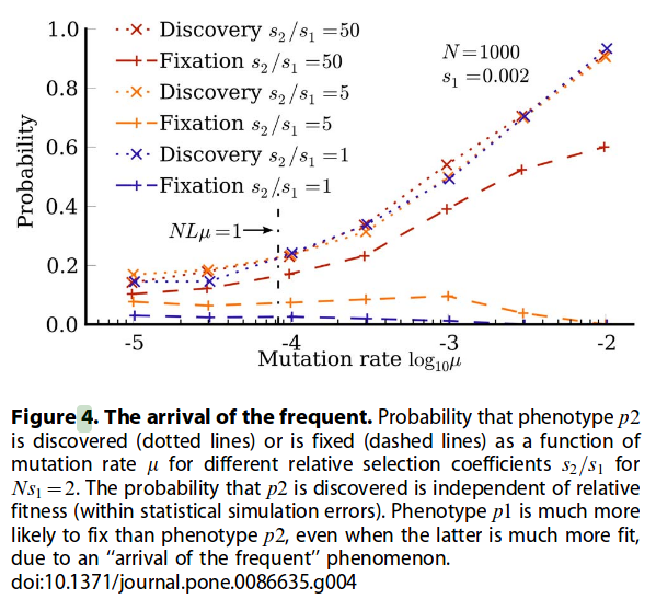
For the monomorphic limit (small mutation rate, in Figure 4.), the probability.....

Summary/Discussion

Genotype-phenotype (GP) maps are observed to be highly biased: Some phenotypes are realised by orders of magnitude more genotypes than most other phenotypes.

Large bias observed in the GP maps translates into a similar order of magnitude variation in the median discovery times $T_p$ for a range of population genetic parameters. However, correlations in the GP map can cause the relation between $T_p$ and phenotype frequency $F_p$ to have large fluctuations (for example, $phi_{pq}$ (which determines $T_p$) can be $0$ even if $F_p$ is quite large).

For the GP mas studied, the strong bias in the GP map leads to a systematic ordering of the median discovery times of alternative phenotypes, an effect that we postulate may hold for other GP maps as well.

The correlations in the RNA GP maps mean that close genotypes have similar neighbourhoods, so that one needs to explore further to reach truly new {genotype neighbourhoods}. This is why the fitting parameter $\gamma$ is smaller than the value expected in the mean-field approx. This is also why for very similar values of $\phi_{pq}4$, there is a range of values of $T_p$ spanning about $1$ order of magnitude. This probably means that it takes up to $\sim 10$ generations to {reach truly novels genotypic neighbourhoods} in the {neutral exploration}. Still, the many orders of magnitude range observed in $\phi_{pq}$ dominates the variation in phenotype discovery times ($T_p$), providing a a posteriori justification for the mean-field approximation.

It is reasonable to expect all these features to arise in other GP maps found in natural (or in artificial systems), including biological systems.

Taken together, these arguments suggest that the vast majority of possible phenotypes may never be found, and thus never fix,even though they may globally be the most fit: Evolutionary search is deeply non-ergodic (I think that this is in the sense that we don't quite reach equilibrium on reasonable time scales, or that the observation time-scales needed for the system to appear ergodic are much larger than those used in experiment. However, this is also true in many other systems like particles in a gas; however, this other system doesn't show the bias needed for the Arrival of the frequent effect).

When Hugo de Vries was advocating for the importance of mutations in evolution, he famously said ‘‘Natural selection may explain the survival of the fittest, but it cannot explain the arrival of the fittest’’ [2]. Here we argue that the fittest may never arrive.Instead evolutionary dynamics can be dominated by the ‘‘arrival of the frequent’’.

Older comments:

So I think what he was talking about is that we can construct a network of phenotypes which is a projection of the network of genotypes via the genotype-phenotype map. Links in the network of genotypes are possible mutations, and all genes have the same degree. However, not all nodes have the same degree in the network of phenotypes.

We can then apply results from network theory of the steady distribution for a random walker on a network.

So this sets a bias on the distribution on the phenotype network.

Over this bias there will be the fitness surface.

https://people.cs.uct.ac.za/~gnitschke/projects/papers/2016-Relationship%20Between%20Evolvability%20and%20Robustness.pdf